Fixing Boundary Violations

2.3 Type II Boundary Constraints

Type II constraints are related to the regression coefficient $\beta$ , which is best illustrated by the centered model

$\begin{equation*} {{y}_{i}}=\boldsymbol{x_{i}^{*}\beta}, \end{equation*}$
where

$\boldsymbol{{x}^{*}}$ refers to the matrix of the independent variables

$\boldsymbol{x_{j}}$ ,

$j=1,\ldots ,m$ , after being centered at the means

${{\bar{x}}_{j}}$ ,

$\begin{equation*} \boldsymbol{x^{*}}=\left( \begin{matrix} \vdots & \vdots & & \vdots \\ 1 & \left( {{x}_{1i}}-{{\bar{x}}_{1}} \right) & \cdots & \left( {{x}_{mi}}-{{\bar{x}}_{m}} \right)\\ \vdots & \vdots & & \vdots \end{matrix} \right). \end{equation*}$

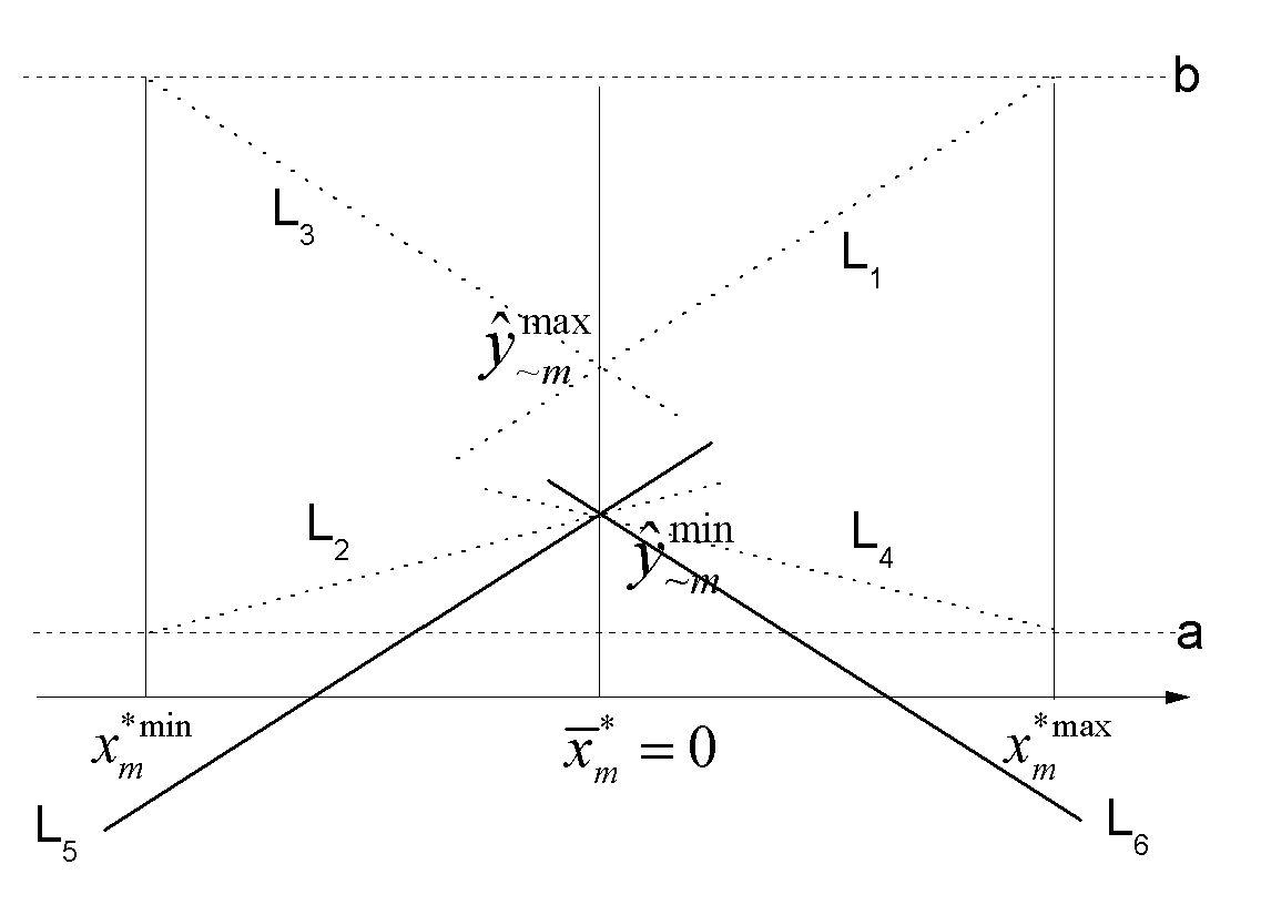
Figure 1 Boundary Constraints of $\beta_{m}$

The constant ${{\hat{\beta }}_{0}}$ now represents the mean estimate of $y_{i}$ when none of the covariates has explanatory power, or represents the baseline predicted value of $y_{i}$ when all covariates are held by the means. Apparently, the boundary constraints of ${{\hat{\beta }}_{0}}$ should be within the truncation interval

$\begin{equation*} a\le {{\hat{\beta }}_{0}}\le b. \end{equation*}$
To discover the possible range of other

${{\hat{\beta }}_{m}}$ , we first hold

${{x}_{m}^{*}}$ at the mean level

$\bar{x}_{m}^{*}$ as Figure 1 shows, and then derive the maximum and minimum of the predicted values,

$\hat{y}_{\sim m}^{\max }$ and

$\hat{y}_{\sim m}^{\min }$ , respectively. The notation "

$\sim$

$m$ " represents the fact that

${{x}_{m}^{*}}$ has no contribution when it is held at the mean. More precisely,

$\hat{y}_{\sim m}^{\max }$ and

$\hat{y}_{\sim m}^{\min }$ can be specified

$\begin{align*} &\hat{y}_{\sim m}^{\max}=\sum\limits_{j=0,j\ne m}{\left(v_{j}^{+} {{\hat{\beta}}_{j}}x_{j}^{*\max}+v_{j}^{-}{{\hat{\beta}}_{j}}x_{j}^{*\min} \right)} \\ &\hat{y}_{\sim m}^{\min}=\sum\limits_{j=0,j\ne m}{\left(v_{j}^{+}{{\hat{\beta}}_{j}}x_{j}^{*\min}+v_{j}^{-} {{\hat{\beta}}_{j}}x_{j}^{*\max} \right)}. \end{align*}$
The upper limit of

$\beta_{m}$ is the flatter positive slope of the line

$L_{1}$ or

$L_{2}$ . The lower limit is the flatter negative slope of the line

$L_{3}$ or

$L_{4}$ . Therefore, the boundary constraints of

${{\hat{\beta }}_{m}}$ can be identified as

$\begin{equation*} \max \left( \frac{a-\hat{y}_{\sim m}^{\min }}{x_{m}^{*\max }},-\frac{\hat{y}_{\sim m}^{\max }-b} {x_{m}^{*\min }} \right)\le {{\hat{\beta }}_{m}}\le \min \left( \frac{b-\hat{y}_{\sim m}^{\max }} {x_{m}^{*\max }},-\frac{\hat{y}_{\sim m}^{\min }-a}{x_{m}^{*\min }} \right). \end{equation*}$
If

$\hat{\beta}_{m}$ takes the steeper slope, such as

$L_{5}$ or

$L_{6}$ shows, it would generate an out-of-bounds predicted value when we vary

${{x}_{m}^{*}}$ from the mean to the maximum or minimum, holding other variables at the baseline level. In this sense, a type II violation can always be translated into a type I violation.

Different centering methods do not generate different estimates of the beta coefficients, except the constant, which is a linear combination of all other beta coefficients and the centered covariate values.⁷ For a truncated regression model with $m$ covariates, there will always be $(2m+2)$ type II boundary constraints, including the constant.

____________________

Footnote

⁷ This rule only applies to a strict linear model. If truncated regression is specified with a nonlinear relationship, such as interaction, different centering methods will generate different results.